In the field of metaheuristic algorithms, experimentation is probably the most important tool to assess and compare the performance of different algorithms. However, most studies limit themselves to presenting the means and standard deviations of the final benchmark results. The objective of this project is to create a web-based application that can provide deeper insights into an algorithm’s behavior and more holistic comparisons with other algorithms. The core concept is to store all data on a web-server and run experiments on a Linux-Cluster. Each experiment will use the same amount of nodes, which provides comparable results of the experiments. The analysis of the created outputs is generated in form of a PDF or XHTML report, containing diagrams and plots with evaluation and a comparison of the tested algorithms. Not only do these concepts enable any user to compare all kinds of optimization algorithms for a certain problem without comparing the machines that the other algorithms were tested on, but also analyze any algorithm’s progress over time.

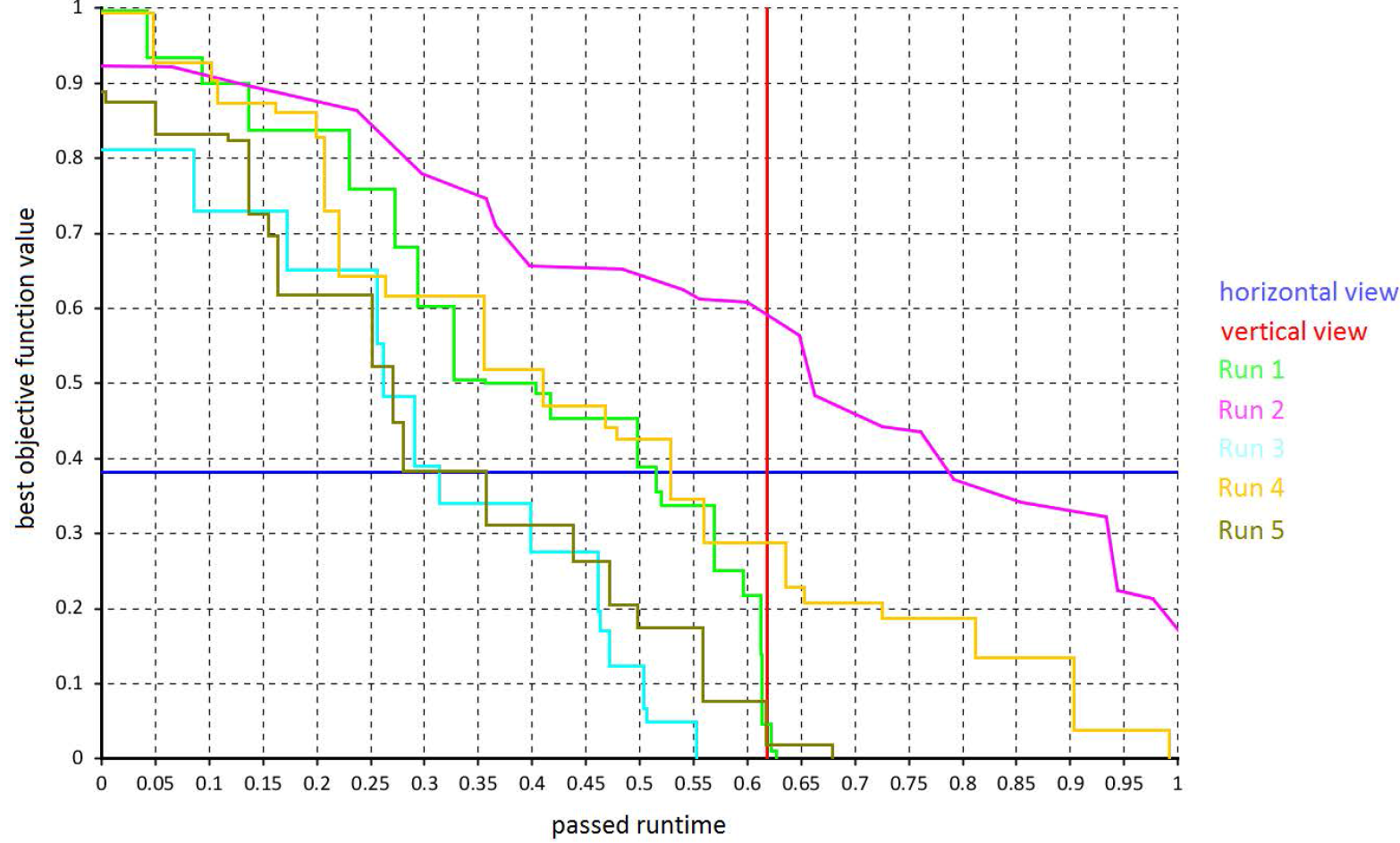
Example for cuts - An example for several runs of an optimization algorithm and the concept of horizontal and vertical cuts. Figure 1 depicts two ways to measure the quality of an algorithm against an objective function (optimal value = 0): the solution value obtained after a fixed run-time (vertical cut in objective value vs. time plot) and the run-time required to achieve a certain solution value (horizontal cut in Figure 1).

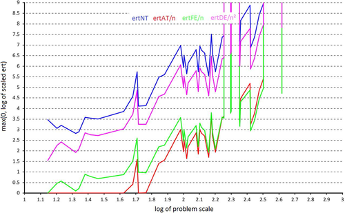
Example ert plots: Figure 2 shows the plot of the Estimated Running Time (ert) to success for different relative goal objective values. The ert denotes the amount of time that passes in expectation until an optimization algorithm reaches a given target objective function value (ft), for the first time. If a run never reaches ft, then all the time spent for this run is added and if no run reaches ft the ert = +∞. The ert is an example of a horizontal-cut performance measure. Each value in the plot is appropriately scaled: the distance evaluations (DEs) scaled by n2, the function evaluations (FEs) scaled by n, the absolute runtime (ATs) by n while the normalized runtime (NTs) does not scaling.

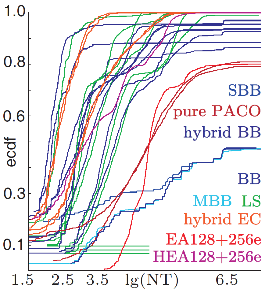
Example ECDF plots: Figure 3 illustrates the ECDF (empirical cumulative distribution functions) comparisons of several algorithms with a goal error of 0.1. for the Traveling Salesman Problem ECDF basically computes the probability to which a run of the algorithm obtains a solution of a certain quality, i.e. F <= Ft. Here, F is the error in the solution obtained and Ft is the maximum desired goal error. In the above example this quality measure (Ft) is kept as 0.1. As is clear from the above figure the ECDF of BB based on the normalized CPU run-time measure NT, increases slowly and never reaches 0.5 for Ft = 0.1. In other words, even a 10% margin cannot be reached in more than half of the runs under the given computational budget. The ECDF curves of BB, MBB and SBB all increase slowly and approach each other as time increases. If we measure time in terms of FEs (function evaluations) instead of (normalized) CPU seconds, we see that the tested BB algorithms can only create relatively few solutions within the granted computational budget and thus, the ECDF stops increasing early.

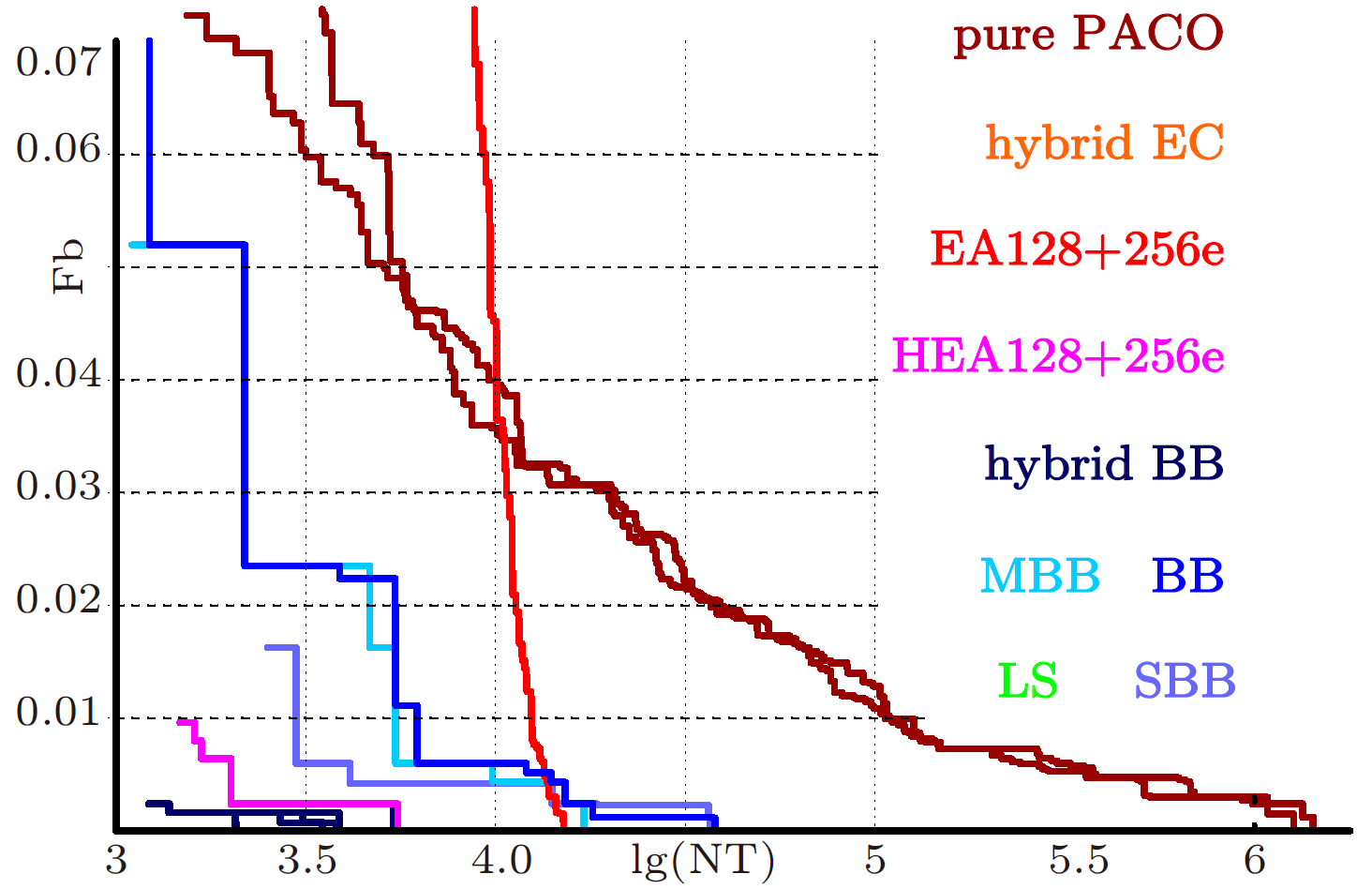
In Figure 4, we see that the BB algorithm can find the optimal solutions for instances with n between 16 and 31 quite rapidly, and for 32 = n < 63, although not as good as LS algorithms, it still can find solutions with Ft = 0.05. As the problem scale increases, however, its performance decreases. While the NT is related to the actual consumed runtime, we can also measure the progress of an algorithm relative to the number of candidate solutions it has constructed, i.e., the number of function evaluation.In Figure 4, we see that the BB algorithm can find the optimal solutions for instances with n between 16 and 31 quite rapidly, and for 32 = n < 63, although not as good as LS algorithms, it still can find solutions with Ft = 0.05. As the problem scale increases, however, its performance decreases. While the NT is related to the actual consumed runtime, we can also measure the progress of an algorithm relative to the number of candidate solutions it has constructed, i.e., the number of function evaluation.
Extended details of our ongoing work can be found
![]() here
here
Partners/Cooperations